Class 6 (Discrete-time linear, time-invariant (LTI) systems)
The sifting or sampling property
Conceptual summary: The sifting property states that we can represent any signal as a weighted sum of shifted impulses . We derive this below.
Representing any signal with impulses
First, we consider a simple property. If we multiply a signal $x[n]$ by shifted impulse $\delta[t-T]$, we notice that $$ x[n]\delta[n-N] = x[N]\delta[n-N] .$$ We get this result because $\delta[n-N]$ is zero everywhere except at time $n = N$. Therefore, only the value at $x[N]$ is expressed in the signal.
We can now expand this idea to the entire signal. Intuitively, we show that we can represent any signal as an infinite, discrete sum of shifted impulses with different amplitudes. Mathematically, this is written as $$ \begin{eqnarray} x[n] &=& \sum_{m=-\infty}^{\infty} x[n] \delta[n - m] \\ &=& \sum_{m=-\infty}^{\infty} x[m] \delta[n - m] . \end{eqnarray} $$ That is, at every $m$, we sample $x[n]$ at $n = m$. In the end, we get back $x[n]$. This is known as the sifting property or the sampling property of an impulse function.
At first glance, this may seem like an exercise in tautology. However, this property is key to understanding linear, time-invariant (LTI) systems.
Understanding LTI Systems
Conceptual summary: Linear, time-invariant (LTI) systems are special because any can be expressed as a weighted sum of shifted impulse responses (the system's output with an impulse input). The weights and shifts are determined by the inputs values. We derive this below.
Step 1: Start with a time-invariant system
Let the input to a time-invariant system $\mathcal{H}\{ \cdot \}$ be an impulse $\delta[n]$. Due to time-invariance, we know that delaying or advancing the impulse will delay or advance the output $h[n]$. Hence, we can say $$\mathcal{H}\{ \delta[n + m] \} = h[n + m].$$
Step 2: Add linearity
To now continue to consider the time-invariant system $\mathcal{H}\{ \cdot \}$ discussed in the previous subsection. If this system is also linear, we will know what output to expect from a sum of two or more different $\delta$ inputs. For example, for the input signal $x[n] = x[m_1] \delta[n + m_1] + x[m_2] \delta[n + m_2]$, the output response would be $$ \begin{eqnarray} \mathcal{H}\{ x[n] \} &=& \mathcal{H}\{ x[m_1] \delta[n + m_1] + x[m_2] \delta[n + m_2] \} \\ &=& \mathcal{H}\{ x[m_1] \delta[n + m_1] \} + \mathcal{H}\{ x[m_2] \delta[n + m_2] \} \quad (\textrm{due to linearity}) \\ &=& x[m_1] \mathcal{H}\{ \delta[n + m_1] \} + x[m_2] \mathcal{H}\{ \delta[n + m_2] \} \quad (\textrm{due to linearity}) \\ &=& x[m_1] \, h[n + m_1] + x[m_2] \, h[n + m_2]. \end{eqnarray} $$
Step 3: Extend with the sampling property
In the previous subsection, we showed that linearity allowed us to determine the output from a sum of two different $\delta$ functions. We can extend this idea to a sum of any number of delta functions. Furthermore, the sampling property tells us that we can represent any signal $x[n]$ as an infinite sum of amplified delta functions. So if we now let $x[n]$ be the input to the linear, time-invariant (LTI) system $\mathcal{H}\{ \cdot \}$, we get $$ \begin{eqnarray} \mathcal{H} \left\{ x[n] \right\} &=& \mathcal{H} \left\{ \sum_{m=-\infty}^{\infty} x[m] \delta[n - m] \right\} \\ &=& \sum_{m=-\infty}^{\infty} x[m] \mathcal{H} \left\{ \delta[n - m] \right\} \quad (\textrm{due to linearity}) \\ &=& \sum_{m=-\infty}^{\infty} x[m] h[n - m] \\ &=& x[n] * h[n] . \end{eqnarray} $$ The result of these steps is known as the convolution sum.
This result shows that we can describe the output of any linear, time-invariant system through the convolution sum. To find the output, we need to know the input signal $x[n]$ and and the impulse response $h[n]$. The function $h[n]$ is the response of the system to an single impulse at time t=0, i.e., $\delta[n]$.
If an impulse response of a system is infinite in duration, we refer to it as an infinite impulse response system. If an impulse response of a system is finite in duration, we refer to it as an finite impulse response system.
Convolution properties
Commutativity $$ x[n] * h[n] = h[n] * x[n]$$
Associativity $$ g[n] * \left(x[n] * h[n] \right) = \left(g[n] * x[n] \right) * h[n] $$
Distributivity $$ g[n] * \left(x[n] + h[n] \right) = g[n] * x[n] + g[n] * h[n] $$
Associativity with scalar multiplication $$ a \left( x[n] * h[n] \right) = \left( a x[n] \right) * h[n] $$
Multiplicative identity $$ x[n] * \delta[n] = x[n] $$
Graphically understanding convolution
Convolution can be seen as a graphical process:
- Plot $x[m]$ with dependent variable $m$
- Plot $h[-m]$ with dependent variable $m$ ($h$ reflected around $m=0$).
- Plot $h[n-m]$ with dependent variable $m$ ($n$ can shift $h[n-m]$ from $-\infty$ (all the way to the left) to $\infty$ (all the way to the right).
- For each shift (i.e. $n$), compute $y[n] = \sum_{m=-\infty}^{\infty} x[m] h[n-m]$ (i.e., multiply $x[m] h[n-m]$ and then sum the result ).
Graphical Convolution Examples
Solving the convolution sum for discrete-time signal can be a bit more tricky than solving the convolution integral. As a result, we will focus on solving these problems graphically. Below are a collection of graphical examples of discrete-time convolution.
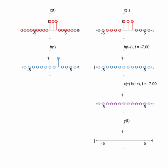
Box and an impulse
$x[n] = u[n] - u[n-3]$
$h[n] = \delta[n - 2]$
$y[n] = x[n] * h[n]$
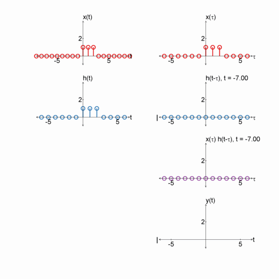
Two boxes
$x[n] = u[n] - u[n-3]$
$h[n] = u[n] - u[n-3]$
$y[n] = x[n] * h[n]$
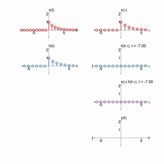
Box and exponential
$x[n] = u[n] - u[n-3]$
$h[n] = e^{(-1/2) n} u[n]$
$y[n] = x[n] * h[n]$

Two exponentials
$x[n] = e^{(-1/2) n} u[n]$
$h[n] = e^{(-1/2) n} u[n]$
$y[n] = x[n] * h[n]$
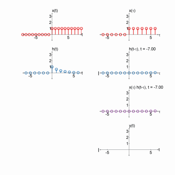
Step function and an exponential
$x[n] = u[n]$
$h[n] = e^{(-1/2) n} u[n]$
$y[n] = x[n] * h[n]$
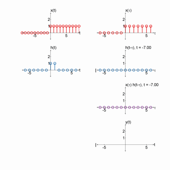
Step function and a box
$x[n] = u[n]$
$h[n] = u[n] - u[n-2]$
$y[n] = x[n] * h[n]$
Additional Resources
- From this course
- From Richard Baraniuk's open textbook
- Discrete Time Convolution
- Properties of Discrete Time Convolution